Cologne Database for Molecular Spectroscopy (CDMS) Queries (astroquery.linelists.cdms)
Getting Started
The CDMS module provides a query interface for the Search and Conversion Form
of the Cologne Database for Molecular Spectroscopy. The module outputs the results that
would arise from the browser form using similar search criteria as the ones
found in the form, and presents the output as a Table. The
module is similar in spirit and content to the JPLSpec module.
Examples
Querying the catalog
The default option to return the query payload is set to False. In the
following examples we have explicitly set it to False and True to show the what
each setting yields:
- group:
shared
>>> from astroquery.linelists.cdms import CDMS
>>> import astropy.units as u
>>> response = CDMS.query_lines(min_frequency=100 * u.GHz,
...                             max_frequency=1000 * u.GHz,
...                             min_strength=-500,
...                             molecule="028503 CO",
...                             get_query_payload=False)
>>> response.pprint(max_width=120)
    FREQ     ERR    LGINT   DR   ELO    GUP  TAG   QNFMT  Ju  Ku  vu ... F3u  Jl  Kl  vl F1l F2l F3l   name  MOLWT Lab
    MHz      MHz   nm2 MHz      1 / cm                               ...                                       u
----------- ------ ------- --- -------- --- ------ ----- --- --- --- ... --- --- --- --- --- --- --- ------- ----- ----
115271.2018 0.0005 -5.0105   2      0.0   3 -28503   101   1  --  -- ...  --   0  --  --  --  --  -- CO, v=0    28 True
   230538.0 0.0005 -4.1197   2    3.845   5 -28503   101   2  --  -- ...  --   1  --  --  --  --  -- CO, v=0    28 True
345795.9899 0.0005 -3.6118   2   11.535   7 -28503   101   3  --  -- ...  --   2  --  --  --  --  -- CO, v=0    28 True
461040.7682 0.0005 -3.2657   2  23.0695   9 -28503   101   4  --  -- ...  --   3  --  --  --  --  -- CO, v=0    28 True
576267.9305 0.0005 -3.0118   2  38.4481  11 -28503   101   5  --  -- ...  --   4  --  --  --  --  -- CO, v=0    28 True
691473.0763 0.0005 -2.8193   2  57.6704  13 -28503   101   6  --  -- ...  --   5  --  --  --  --  -- CO, v=0    28 True
 806651.806  0.005 -2.6716   2  80.7354  15 -28503   101   7  --  -- ...  --   6  --  --  --  --  -- CO, v=0    28 True
   921799.7  0.005  -2.559   2 107.6424  17 -28503   101   8  --  -- ...  --   7  --  --  --  --  -- CO, v=0    28 True
The following example, with get_query_payload = True, returns the payload:
- group:
shared
>>> response = CDMS.query_lines(min_frequency=100 * u.GHz,
...                             max_frequency=1000 * u.GHz,
...                             min_strength=-500,
...                             molecule="028503 CO",
...                             get_query_payload=True)
>>> print(response)
{'MinNu': 100.0, 'MaxNu': 1000.0, 'UnitNu': 'GHz', 'StrLim': -500, 'temp': 300, 'logscale': 'yes', 'mol_sort_query': 'tag', 'sort': 'frequency', 'output': 'text', 'but_action': 'Submit', 'Molecules': '028503 CO'}
The units of the columns of the query can be displayed by calling
response.info:
- group:
shared
>>> response = CDMS.query_lines(min_frequency=100 * u.GHz,
...                             max_frequency=1000 * u.GHz,
...                             min_strength=-500,
...                             molecule="028503 CO",
...                             get_query_payload=False)
>>> print(response.info)
<Table length=8>
 name  dtype    unit     class     n_bad
----- ------- ------- ------------ -----
 FREQ float64     MHz       Column     0
  ERR float64     MHz       Column     0
LGINT float64 nm2 MHz       Column     0
   DR   int64               Column     0
  ELO float64  1 / cm       Column     0
  GUP   int64               Column     0
  TAG   int64               Column     0
QNFMT   int64               Column     0
   Ju   int64               Column     0
   Ku   int64         MaskedColumn     8
   vu   int64         MaskedColumn     8
  F1u   int64         MaskedColumn     8
  F2u   int64         MaskedColumn     8
  F3u   int64         MaskedColumn     8
   Jl   int64               Column     0
   Kl   int64         MaskedColumn     8
   vl   int64         MaskedColumn     8
  F1l   int64         MaskedColumn     8
  F2l   int64         MaskedColumn     8
  F3l   int64         MaskedColumn     8
 name    str7               Column     0
MOLWT   int64       u       Column     0
  Lab    bool               Column     0
These come in handy for converting to other units easily, an example using a simplified version of the data above is shown below:
- group:
shared
>>> print(response['FREQ', 'ERR', 'ELO'])
     FREQ     ERR     ELO
     MHz      MHz    1 / cm
 ----------- ------ --------
 115271.2018 0.0005      0.0
    230538.0 0.0005    3.845
 345795.9899 0.0005   11.535
 461040.7682 0.0005  23.0695
 576267.9305 0.0005  38.4481
 691473.0763 0.0005  57.6704
  806651.806  0.005  80.7354
    921799.7  0.005 107.6424
>>> response['FREQ'].quantity
 <Quantity [115271.2018, 230538.    , 345795.9899, 461040.7682, 576267.9305,
            691473.0763, 806651.806 , 921799.7   ] MHz>
>>> response['FREQ'].to('GHz')
 <Quantity [115.2712018, 230.538    , 345.7959899, 461.0407682, 576.2679305,
            691.4730763, 806.651806 , 921.7997   ] GHz>
The parameters and response keys are described in detail under the Reference/API section.
Retrieving Complete Molecule Catalogs
If you need all spectral lines for a specific molecule without filtering by
frequency range or strength, or if there is a problem with the query tool’s
version of a table (which occurs for some molecules with particularly
complicated quantum numbers), you can use the get_molecule method. This
method retrieves the complete catalog file for a given molecule using its
6-digit identifier.
>>> from astroquery.linelists.cdms import CDMS
>>> # Retrieve all lines for CO (molecule tag 028503)
>>> table = CDMS.get_molecule('028503')
>>> print(f"Retrieved {len(table)} lines for CO")
Retrieved 95 lines for CO
>>> table[:5].pprint(max_width=120)
    FREQ     ERR    LGINT   DR   ELO   GUP  TAG   QNFMT  Q1  Q2  Q3 ...  Q6  Q7  Q8  Q9 Q10 Q11 Q12 Q13 Q14 MOLWT Lab
    MHz      MHz   nm2 MHz      1 / cm                              ...                                       u
----------- ------ ------- --- ------- --- ------ ----- --- --- --- ... --- --- --- --- --- --- --- --- --- ----- ----
115271.2018 0.0005 -5.0105   2     0.0   3 -28503   101   1  --  -- ...  --   0  --  --  --  --  --  --  --    28 True
   230538.0 0.0005 -4.1197   2   3.845   5 -28503   101   2  --  -- ...  --   1  --  --  --  --  --  --  --    28 True
345795.9899 0.0005 -3.6118   2  11.535   7 -28503   101   3  --  -- ...  --   2  --  --  --  --  --  --  --    28 True
461040.7682 0.0005 -3.2657   2 23.0695   9 -28503   101   4  --  -- ...  --   3  --  --  --  --  --  --  --    28 True
576267.9305 0.0005 -3.0118   2 38.4481  11 -28503   101   5  --  -- ...  --   4  --  --  --  --  --  --  --    28 True
The molecule identifier must be a number that can be converted to a 6-digit string.
The returned table includes metadata from the species table:
>>> table = CDMS.get_molecule(28503)
>>> print(table.meta['molecule'])
CO, v=0
>>> print(table.meta['Name'])
CO, v = 0
Looking Up More Information from the partition function file
If you have found a molecule you are interested in, the tag column in the
results provides enough information to access specific molecule information
such as the partition functions at different temperatures. Keep in mind that a
negative tag value signifies that the line frequency has been measured in the
laboratory but not in space
>>> import matplotlib.pyplot as plt
>>> from astroquery.linelists.cdms import CDMS
>>> result = CDMS.get_species_table()
>>> mol = result[result['tag'] == 28503]
>>> mol.pprint(max_width=160)
 tag  molecule    Name   #lines lg(Q(1000)) lg(Q(500)) lg(Q(300)) ... lg(Q(9.375)) lg(Q(5.000)) lg(Q(2.725)) Ver. Documentation Date of entry    Entry
----- -------- --------- ------ ----------- ---------- ---------- ... ------------ ------------ ------------ ---- ------------- ------------- -----------
28503  CO, v=0 CO, v = 0     95      2.5595     2.2584     2.0369 ...       0.5733       0.3389       0.1478    1   e028503.cat     Oct. 2000 w028503.cat
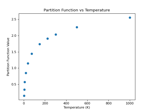
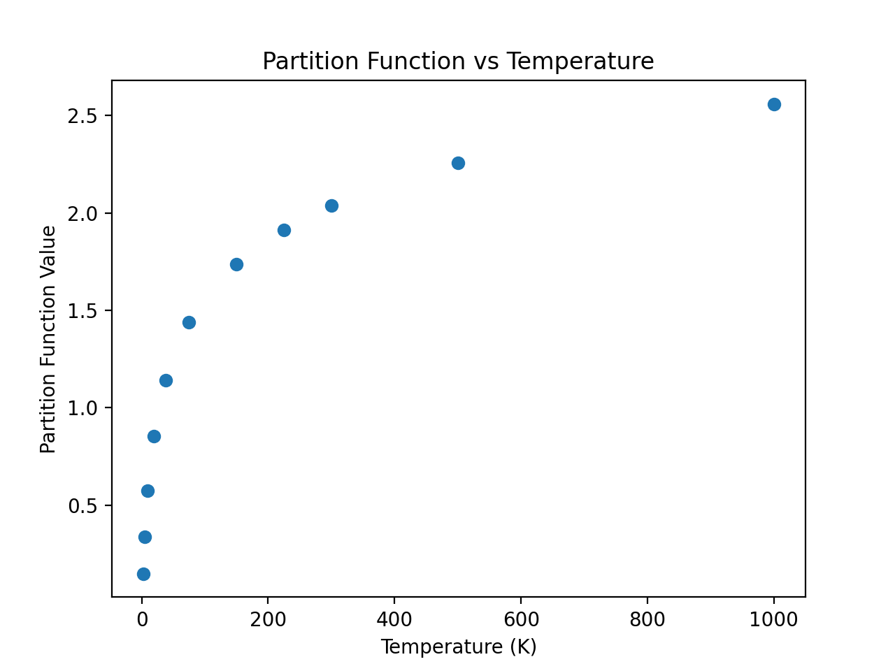
One of the advantages of using CDMS is the availability in the catalog of the partition function at different temperatures for the molecules (just like for JPL). As a continuation of the example above, an example that accesses and plots the partition function against the temperatures found in the metadata is shown below:
>>> import numpy as np
>>> keys = [k for k in mol.keys() if 'lg' in k]
>>> temp = np.array([float(k.split('(')[-1].split(')')[0]) for k in keys])
>>> part = list(mol[keys][0])
>>> plt.scatter(temp, part)
>>> plt.xlabel('Temperature (K)')
>>> plt.ylabel('Partition Function Value')
>>> plt.title('Partition Function vs Temperature')
(Source code, png, hires.png, pdf)

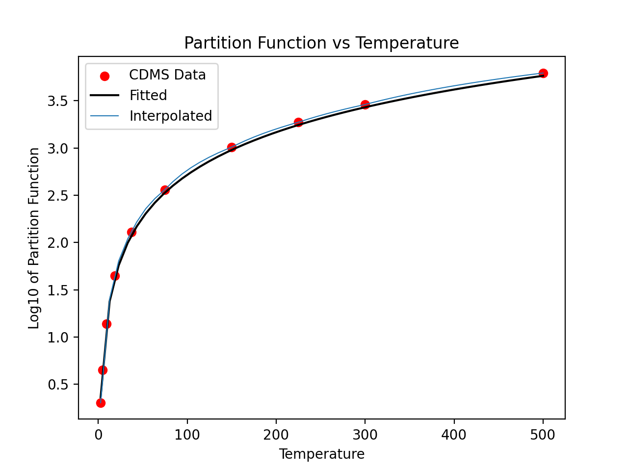
For non-linear molecules like H2CO, curve fitting methods can be used to
calculate production rates at different temperatures with the proportionality:
a*T**(3./2.). Calling the process above for the H2CO molecule (instead of
for the CO molecule) we can continue to determine the partition function at
other temperatures using curve fitting models:
>>> import numpy as np
>>> import matplotlib.pyplot as plt
>>> from astroquery.linelists.cdms import CDMS
>>> from scipy.optimize import curve_fit
...
>>> result = CDMS.get_species_table()
>>> mol = result[result['tag'] == 30501] #do not include signs of tag for this
...
>>> def f(T, a):
        return np.log10(a*T**(1.5))
>>> keys = [k for k in mol.keys() if 'lg' in k]
>>> def tryfloat(x):
...     try:
...        return float(x)
...     except:
...        return np.nan
>>> temp = np.array([float(k.split('(')[-1].split(')')[0]) for k in keys])
>>> part = np.array([tryfloat(x) for x in mol[keys][0]])
>>> param, cov = curve_fit(f, temp[np.isfinite(part)], part[np.isfinite(part)])
>>> print(param)
# array([0.51865074])
>>> x = np.linspace(2.7,500)
>>> y = f(x,param[0])
>>> plt.scatter(temp,part,c='r')
>>> plt.plot(x,y,'k')
>>> plt.title('Partition Function vs Temperature')
>>> plt.xlabel('Temperature')
>>> plt.ylabel('Log10 of Partition Function')
(Source code, png, hires.png, pdf)
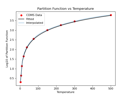
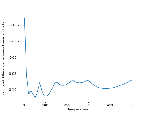
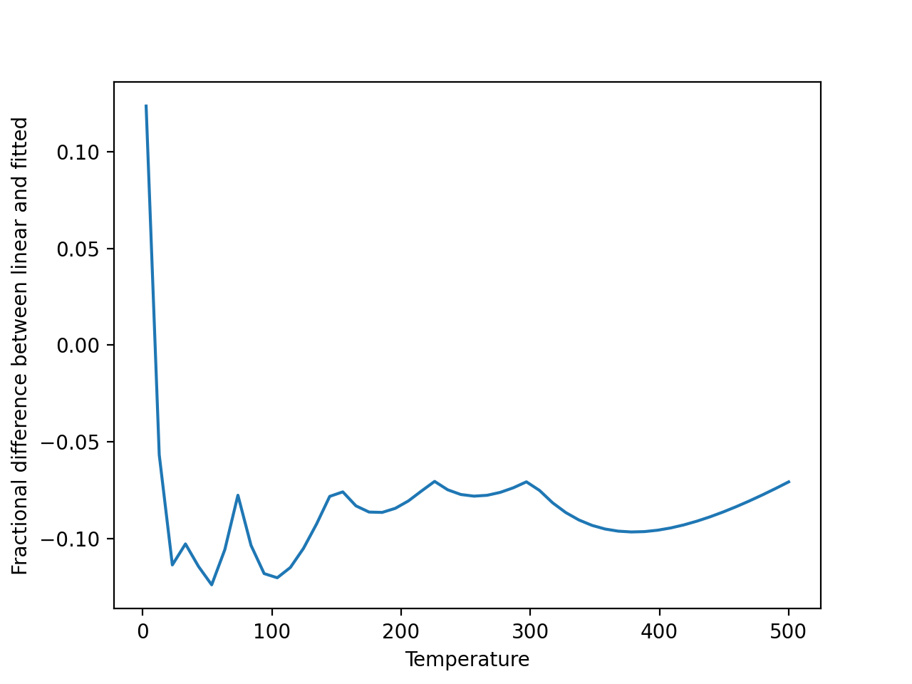
We can then compare linear interpolation to the fitted interpolation above:
>>> interp_Q = np.interp(x, temp, 10**part)
>>> plt.plot(x, (10**y-interp_Q)/10**y)
>>> plt.xlabel("Temperature")
>>> plt.ylabel("Fractional difference between linear and fitted")
(Source code, png, hires.png, pdf)

Linear interpolation is a good approximation, in this case, for any moderately high temperatures, but is increasingly poor at lower temperatures. It can be valuable to check this for any given molecule.
Querying the Catalog with Regexes and Relative names
The regular expression parsing is analogous to that in
astroquery.linelists.jplspec. See Querying the Catalog with Regexes and Relative names.
Handling Malformatted Molecules
There are some entries in the CDMS catalog that get mangled by the query tool, but the underlying data are still good. This seems to affect primarily those molecules with excessive numbers of quantum numbers such as H2NC.
Troubleshooting
If you are repeatedly getting failed queries, or bad/out-of-date results, try clearing your cache:
>>> from astroquery.linelists.cdms import CDMS
>>> CDMS.clear_cache()
If this function is unavailable, upgrade your version of astroquery.
The clear_cache function was introduced in version 0.4.7.dev8479.
Reference/API
astroquery.linelists.cdms Package
CDMS catalog
Cologne Database for Molecular Spectroscopy query tool
Classes
|
CDMS line list query class |
|
Configuration parameters for |